Fri 19 August 2016
Sorting Algorithm Performance
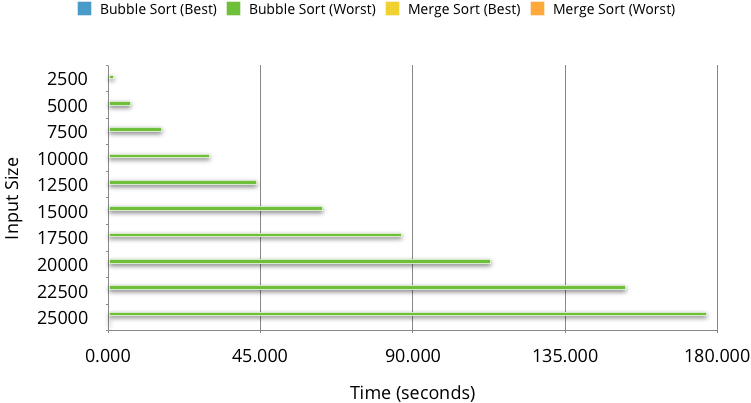
At it's most basic, we can see some algorithms are clearly just faster than others, for a bunch of input sizes we can compare best (Already sorted) and worst (sorted backwards) case times (in seconds) for two common-place algorithms (bubble-sort and merge-sort).
Here's the theory:
| | Best | Average | Worst | |---|---|---|---|---| | Bubble Sort | Ω(n log(n)) | Θ(n^2) | O(n^2) | | Merge Sort | Ω(n log(n)) | Θ(n log(n)) | O(n log(n)) |
In case you aren't familiar with these algorithms, they are some of the most basic taught to first year computer science classes. Bubble sort will loop over the array in-place, swapping pairs of items one by one, until a complete iteration of the array does not perform any swaps. Merge sort on the other hand, uses divide and conquer to break the array into two pairs recurisvely and building a new array.
| Inputs | Bubble Sort (Best) | Bubble Sort (Worst) | Merge Sort (Best) | Merge Sort (Worst) |
|---|---|---|---|---|
| 2500 | 0.001 | 1.735 | 0.033 | 0.037 |
| 5000 | 0.001 | 6.845 | 0.089 | 0.088 |
| 7500 | 0.001 | 15.774 | 0.120 | 0.104 |
| 10000 | 0.002 | 29.932 | 0.137 | 0.126 |
| 12500 | 0.002 | 43.882 | 0.193 | 0.175 |
| 15000 | 0.002 | 63.401 | 0.211 | 0.202 |
| 17500 | 0.002 | 86.674 | 0.255 | 0.229 |
| 20000 | 0.003 | 113.058 | 0.297 | 0.278 |
| 22500 | 0.004 | 153.131 | 0.315 | 0.308 |
| 25000 | 0.005 | 176.978 | 0.351 | 0.437 |
Some things are easier to see in a graph, so have a look.
Searching Algorithm Performance
Here's a very common use case, we need to match two sets of related data. It could be displaying a list of students enrolled in each course from a list of enrolments.